17 Min to complete

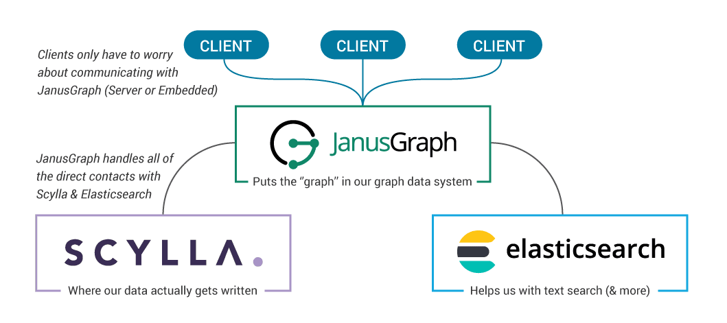
This lesson will teach you how to deploy a Graph Data System, using JanusGraph and ScyllaDB as the underlying data storage layer.
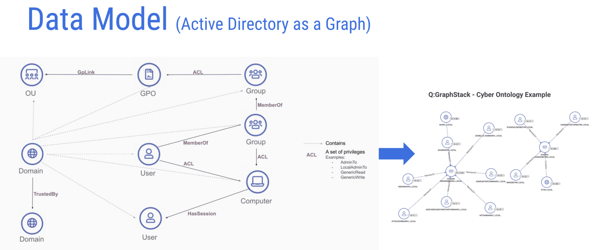
A graph data system (or graph database) is a database that uses a graph structure with nodes and edges to represent data. Edges represent relationships between nodes, and these relationships allow the data to be linked and for the graph to be visualized. It’s possible to use different storage mechanisms for the underlying data, and this choice affects the performance, scalability, ease of maintenance, and cost.
Common use cases for graph databases are knowledge graphs, recommendation applications, social networks, and fraud detection.
JanusGraph is a scalable open-source graph database optimized for storing and querying graphs containing billions of vertices and edges distributed across a multi-machine cluster. It stores graphs in adjacency list format, which means that a graph is stored as a collection of vertices with their edges and properties.
JanusGraph natively supports the graph traversal language Gremlin. Gremlin is a part of Apache TinkerPop and is developed and maintained separately from JanusGraph. Many graph databases support it, and by using it, users avoid vendor lock-in as their applications can be migrated to other graph databases. You can learn more about the architecture on the JanusGraph Documentation page.
JanusGraphs supports ElasticSearch as an indexing backend. ElasticSearch is a search and analytics engine based on Apache Lucene. Using ElasticSearch is not in the scope of this lesson, if you want to see it in a future lesson, drop me a message (#scylla-university channel on slack).
This lesson presents a step-by-step, hands-on example for deploying JanusGraph and performing some basic operations. Here are the main steps in the lesson:
- Spinning up a virtual machine on AWS
- Installing the prerequisites
- Running the JanusGraph server (using Docker)
- Running a Gremlin Console to connect to the new server (also in Docker)
- Spinning up a three-node ScyllaDB Cluster and setting it as the data storage for the JanusGraph server
- Performing some basic graph operations
Since there are many moving parts to setting up JanusGraph and lots of options, the lesson goes over each step in the setup process. It uses AWS, but you can follow through with the example with another cloud provider or with a local machine.
Note that this example is for training purposes only, and in production, things should be done differently. For example, each ScyllaDB node should be run on a single server.
Transactional and Analytical Workloads
In the next part, you’ll spin up a three-node ScyllaDB cluster which you’ll then use as a data storage backend for JanusGraph. The data storage layer for JanusGraph is pluggable. Some options for the data storage layer are Apache HBase, Google Cloud Bigtable, Oracle Berkeley DB Java Edition, Apache Cassandra, and ScyllaDB. The storage backend you use for your application is extremely important. By using ScyllaDB, you’ll get low and consistent latency, high availability, up to x10 throughput, ease of use, and a highly scalable system.
A group at IBM compared using ScyllaDB as the JanusGraph storage backend vs. Apache Cassandra and HBase. They found that ScyllaDB displayed nearly 35% higher throughput when inserting vertices than HBase and almost 3X Cassandra’s throughput. ScyllaDB’s throughput was 160% better than HBase and more than 4X that of Cassandra when inserting edges. ScyllaDB performed 72% better than Cassandra in a query performance test and nearly 150% better than HBase.
With graph data systems, just like with any data system, you can separate your workloads into two categories – transactional and analytical. JanusGraph follows the Apache TinkerPop project’s approach to graph computation. The Gremlin graph traversal language allows us to traverse a graph, traveling from vertex to vertex via the connecting edges. You can use the same approach for both OLTP and OLAP workloads.
Transactional workloads begin with a small number of vertices (found with the help of an index) and then traverse across a reasonably small number of edges and vertices to return a result or add a new graph element. You can describe these transactional workloads as graph local traversals. The goal of these traversals is to minimize latency.
Analytical workloads require traversing a substantial portion of the vertices and edges in the graph to find our answer. Many classic analytical graph algorithms fit into this bucket. These are graph global traversals, and the goal with these traversals is to maximize throughput.
System Setup
Launch an AWS EC2 Instance
Start by spinning up a t2.large Amazon Linux machine. From the EC2 console, select Instances and Launch Instances. In the first step choose the “Amazon Linux 2 AMI (HVM) – Kernel 5.10, SSD Volume Type – ami-008e1e7f1fcbe9b80 (64-bit x86)” AMI. In the secdond step, select t2.xlarge. The reason for using a t2.xlarge machine is that we’re running a few docker instances on the same server, and it requires some resources. Change the storage to 16GB.
Once the machine is running, connect to it using SSH. In the command below, replace the path to your key pair and the public DNS name of your instance.
ssh -i ~/Downloads/aws/xxx.pem [email protected]Next, make sure all your packages are updated:
sudo yum updateInstall Java
JanusGraph requires Java. To install Java and its prerequisites, run:
sudo yum install javaRun the following command to make sure the installation succeeded:
java -versionJanusGraph required the $JAVA_HOME environment variable to be set, and it also needs to be added to the $PATH. This isn’t automatically set when installing Java. So you’ll set it manually.
Locate the Java installation location by running:
sudo update-alternatives --config javaCopy the path to the Java Installation. Now, edit the .bashrc file found in the home directory of the ec2-user user, and add the two lines below to the file, replacing the path with the one you copied, without the /bin/java at the end.
export JAVA_HOME="/usr/lib/jvm/java-17-amazon-corretto.x86_64"PATH=$JAVA_HOME/bin:$PATHSave the file and run the following command:
source .bashrcMake sure the environment variables were set:
echo $JAVA_HOMEecho $PATHInstall Docker
Next, since you’ll be running JanusGraph and ScyllaDB in Docker containers, install docker and its prerequisites:
sudo yum install dockerStart the Docker service:
sudo service docker startand (optionally) to ensure that the Docker daemon starts after each system reboot:
sudo systemctl enable dockerAdd the current user (ec2-user) to the docker group so you can execute Docker commands without using sudo:
sudo usermod -a -G docker ec2-userTo activate the changes to the groups, run:
newgrp dockerFinally, make sure that the Docker engine was successfully installed by running the hello-world image:
docker run hello-worldInstall Docker Compose
Install Docker Compose by copying the appropriate docker-compose binary from GitHub:
sudo curl -L https://github.com/docker/compose/releases/download/1.22.0/docker-compose-$(uname -s)-$(uname -m) -o /usr/local/bin/docker-composeChange the permissions after the download:
sudo chmod +x /usr/local/bin/docker-composeNext, verify that you can now run it:
docker-compose versionDeploying JanusGraph with ScyllaDB as the Data Storage Backend
There are a few options for how to deploy JanusGraph. In this lesson, you’ll deploy JanusGraph using a docker container to simplify the process. Keep in mind that the configuration of JanusGraph, when using Docker is different than when running it directly.
The setup shown here is not recommended for production. Among other things, in production, you should not run ScyllaDB and JanusGraph on the same machine.
To learn about other ways of deploying JanusGraph read the Installation Guide.
If you haven’t done so yet, download the MMS example files, which include the docker-compose that you’ll use to spin up the ScyllaDB cluster and the JanusGraph server:
git clone https://github.com/scylladb/scylla-code-samples.gitcd scylla-code-samples/mms/janusgraph/Once you have the docker-compose file and docker-compose is setup, run it:
docker-compose -f ./docker-compose-cql.yml up -dThis starts a three-node ScyllaDB cluster as well as a JanusGraph server.
Wait a minute or so and check that the ScyllaDB cluster has three nodes up and running in the UN status:
docker exec -it scylla-node1 nodetool statusNext, make sure the JanusGraph server is running and is in a healthy state:
docker ps -aIf the JanusGraph server is in “unhealthy” mode, check the logs (docker logs janusgraph-server). This might happen if the server starts before the ScyllaDB cluster is up and running. In such a case, restart the janusgraph server (docker restart janusgraph-server).
Gremlin Console and Graph Queries
Gremlin is a graph traversal query language developed by Apache TinkerPop. It works for OLTP and OLAP type traversals and supports multiple graph systems. JanusGraph, Neo4j, and Hadoop are some examples.
Run the Gremlin console, and link it to the already running server container. In the following command, the docker network is specified. Make sure you use the right network, which can be different. To see the networks use the docker network ls command.
docker run --rm --network ec2-user_web --link janusgraph-server:janusgraph -e GREMLIN_REMOTE_HOSTS=janusgraph -it janusgraph/janusgraph:latest ./bin/gremlin.sh
Now in the gremlin console, connect to the server:
:remote connect tinkerpop.server conf/remote.yamlThe following command tells the console to send all subsequent commands to the current remote connection:
:remote consoleScyllaDB is configured as the data storage. Verify this (g is the graph traversal source):
gNow you can perform some basic queries. Make sure the graph is empty, to begin with:
g.V().count()Add two vertices
g.addV('person').property('name', 'guy')g.addV('person').property('name', 'john')And make sure they were added:
g.V().values('name')Summary
You learned how to deploy JanusGraph with ScyllaDB as the underlying database in this lesson. There are different ways to deploy JanusGraph and ScyllaDB. To simplify the lesson, it uses Docker. The main steps were: Spinning up a virtual machine on AWS, running the JanusGraph server, running a Gremlin Console to connect to the new server, spinning up a three-node ScyllaDB cluster, and setting it as the data storage for the JanusGraph server, and performing some basic graph operations.
You can learn more about using JanusGraph with ScyllaDB from this real-world Cybersecurity use case. Another use case is Zeotap, which built a graph of twenty billion IDs on ScyllaDB and JanusGraph, which they use for their customer intelligence platform. In terms of performance, a group at IBM compared using ScyllaDB as the JanusGraph storage backend vs. Apache Cassandra and HBase. They found that ScyllaDB displayed nearly 35% higher throughput when inserting vertices than HBase and almost 3X Cassandra’s throughput. ScyllaDB’s throughput was 160% better than HBase and more than 4X that of Cassandra when inserting edges. ScyllaDB performed 72% better than Cassandra in a query performance test and nearly 150% better than HBase.
These ScyllaDB benchmarks compare its performance to Cassandra, DynamoDB, Bigtable, and CockroachDB.